Visualising 19th Century Reading in Australia
I’ve recently spent a bit of time collaborating with my wife on a research project. Research collaboration by couples is not new but given that Julieanne is a lecturer in the English program and I’m part of the computer sciences laboratory, this piece of joint research is a little unusual.
The rest of this post describes the intersection of our interests — data from the Australian Common Reader Project — and the visualisation tool I wrote to explore it. The tool itself is based on a simple application of linear Principal Component Analysis (PCA). I’ll attempt to explain it here in such a way that readers who have not studied this technique might still be able to make use of the tool.
The Australian Common Reader Project
One of Julieanne’s research interests is the Australian audience of the late 19th and early 20th centuries. As part of her PhD, she made use of an amazing database that is part of the Australian Common Reader Project — a project that has collected and entered library borrowing records from Australian libraries along with annotations about when books were borrowed, their genres, borrower occupations, author information, etc. This sort of information makes it possible for Australian literature and cultural studies academics to ask empirical questions about Australian readers’ relationship with books and periodicals.
Ever on the lookout for interesting data sets, I suggested that we apply some basic data analysis tools to the database to see what kind of relationships between books and borrowers we might find. When asked if we could have access to the database, Tim Dolin graciously agreed and enlisted Jason Ensor to help with our technical questions.
Books and Borrowers
After an initial inspection, my first thought was to try to visualise the similarity of the books in the database as measured by the number of borrowers they have in common. The full database contains 99,692 loans of 7,078 different books from 11 libraries by one of the 2,642 people. To make this more manageable, I focused on books that had at least 20 different borrowers and only considered people who had borrowed one of these books. This distilled the database down to a simple table with each row representing one of 1,616 books and each column representing one of 2,473 people.
|
Book ID | Borrower ID | |||
|---|---|---|---|---|
| 1 | 2 | … | 2,473 | |
| 1 | 1 | 0 | … | 1 |
| 2 | 1 | 1 | … | 0 |
| 3 | 0 | 0 | … | 1 |
| … | … | … | … | … |
| 1,616 | 1 | 1 | … | 1 |
Conceptually, each cell in the table contains a 1 if the person associated with the cell’s column borrowed the book associated with the cell’s row. If there was no such loan between a given book and borrower the corresponding cell contains a 0. For example, Table 1 shows that book 2 was borrowed (at least once) by borrower 1 but never by borrower 2,473.
Book Similarity
The table view of the books and their borrowers does not readily lend itself to insight. The approach we took to get a better picture of this information was to plot each book as a point on a graph so that similar books are placed closer together than dissimilar books. To do this a notion of what “similar books” is required.
Mathematically, row \(i\) of Table 1 can be represented as a vector \(\mathbf{b}_i\) of 1s and 0s. The value of the cell in the \(j\)th column of that row will be denoted \(b_{i,j}\). For example, the 2nd row in the table can be written as the vector \(\mathbf{b}_2 = (1,1,\ldots,0)\) and the value in its first column is \(b_{2,1} = 1\).
A crude measure of the similarity between book 1 and book 2 can be computed from this table by counting how many borrowers they have in common. That is, the number of columns that have a 1 in the row for book 1 and the row for book 2.
In terms of the vector representation, this similarity measure is simply the “inner product” between \(\mathbf{b}_1\) and \(\mathbf{b}_2\) and is written \(\left<\mathbf{b}_1,\mathbf{b}_2\right> = b_{1,1}b_{2,1} + \cdots + b_{1,N}b_{2,N}\) where N = 2,473 is the total number of borrowers.
It turns out that simply counting the number of borrowers two books is not a great measure of similarity. The problem is that two very popular books, each with 100 borrowers, that only share 10% of their borrowers would be considered as similar as two books, each with 10 readers, that share all of their borrowers. An easy way to correct this is to “normalise” the borrower counts by making sure the similarity of a book with itself is always equal to 1. A common way of doing this is by dividing the inner product of two books by the “size” of each of the vectors for those books.
Mathematically, we will denote the size of a book vector \(\mathbf{b}_i\) as \(\|\mathbf{b}_i\| = \sqrt{\left<\mathbf{b}_i,\mathbf{b}_i\right>}\). The similarity between two books then becomes: \[ \text{sim}(\mathbf{b}_i,\mathbf{b}_j) = \frac{\left< \mathbf{b}_i,\mathbf{b}_j \right>}{\|\mathbf{b}_i\| \|\mathbf{b}_j\|} \]
Principal Component Analysis
Now that we have a similarity measure between books the idea is to create a plot of points — one per book — so that similar books are placed close together and dissimilar books are kept far apart.
A standard technique for doing this is Principal Component Analysis. Intuitively, this technique aims to find a way of reducing the number of coordinates in each book vector in such a way that when the similarity between two books is computed using these smaller vectors it is as close as possible to the original similarity. That is, PCA creates a new table that represents books in terms of only two columns.
|
Book ID | PCA ID | |
|---|---|---|
| 1 | 2 | |
| 1 | –8.2 | 2.3 |
| 2 | 0.4 | –4.3 |
| 3 | –1.3 | –3.7 |
| … | … | … |
| 1,616 | 2.2 | –5.6 |
Table 2 gives an example of the book table after PCA that reduces the book vectors (rows) from 2,473 to two entries. The PCA columns cannot be as easily interpreted as the borrowers columns in Table 1 but the values in the columns are such that the similarity of the books in Table 2 are roughly as similar as if the values in Table 1 were used. That is, if \(\mathbf{c}_1 = (-8.2,2.3)\) and \(\mathbf{c}_2=(0.4,-4.3)\) are the vectors for the first two rows of Table 2 then \(\text{sim}(\mathbf{c}_1,\mathbf{c}_2)\) would be close to \(\text{sim}(\mathbf{b}_1,\mathbf{b}_2)\), the similarity of the first two rows in Table 1.1
Visualising the Data
Figure 1 shows a plot of the PCA reduced book data. Each circle represents one of the 1,616 books, plotted according to the coordinates in a table like Table 2. The size of each circle indicates how many borrowers each book had and its colour indicates which library the book belongs to.2
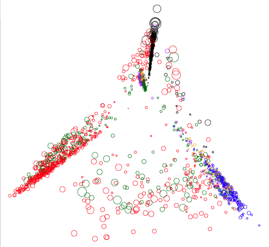
Figure 1: A PCA plot of all the books in the ACRP database coloured according to which library they belong to. The size of each circle indicates the number of borrowers of the corresponding book.
One immediate observation is that books are clustered according to which library they belong to. This is not too surprising since the books in a library limit what borrowers from that library can read. This means it is likely that two voracious readers that frequent the same library will read the same books. This, in turn, will mean the similarity of two books from a library will be higher than books from different libraries as there are very few borrowers that use more than one library.
Drilling Down and Interacting
To get a better picture of the data, we decided to focus on books from a single library to avoid this clustering. The library we focused on was the Lambton Miners’ and Mechanics’ Institute in New South Wales. This library had the largest number of loans (20,253) and so was most likely to have interesting similarity data.
There are a total of 789 books in the Lambton institute and 469 borrowers of those books. A separate PCA reduction was performed on this restricted part of the database to create a plot of only the Lambton books.
To make it easier to explore this data, I wrote a simple tool that allows a viewer to interact with the PCA plot. A screenshot from this tool is shown in Figure 2. Once again, larger circles represent books with a larger number of borrowers.
Clicking on this link will open a new window and, after a short delay, the tool will run.
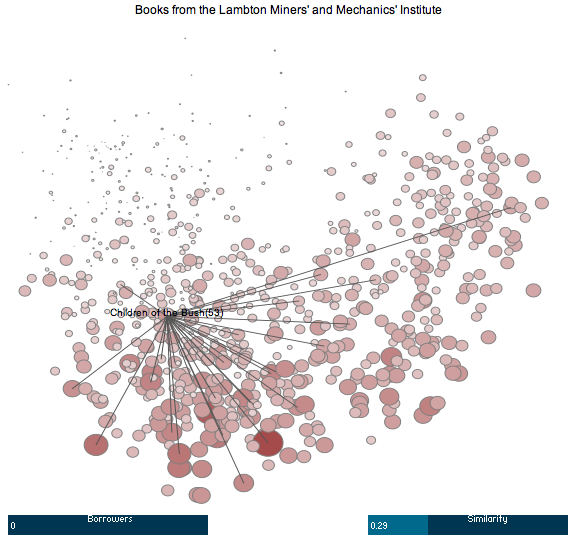
Figure 2: A screenshot of the ACRP visualisation tool showing books from the Lambton Institute. Click the image to run the tool in a new window.
Instructions describing how to use the tool can be found below it. In a nutshell: hovering over a circle will reveal the title of the book corresponding to that circle; clicking on a circle will draw lines to its most similar neighbours; altering the “Borrowers” bar will only show books with at least that many borrowers; and altering the “Similarity” bar will only draw lines to books with at least that proportion of books in common.
Future Work and Distant Reading
Julieanne and I are still at the early stages of our research using the ACRP database. The use of PCA for visualisation was a first step in our pursuit of what Franco Moretti calls “distant reading” — looking at books as objects and how they are read rather than the “close reading” of the text of individual books.
Now that we have this tool, we are able to quickly explore relationships between these books based on the reading habits of Australians at the turn of the century. Of course, there are many caveats that apply to any patterns we might see in these plots. For instance, the similarity between books is only based on habits of a small number of readers and will be influenced by the peculiarities of the libraries and the books they choose to buy. For this reason, these plots are not intended to provide conclusive answers to questions we might.
Instead we hope that exploring the ACRP database in this way will lead us to interesting questions about particular pairs or groups of books that can be followed up by a more thorough analysis of their readers, their text as well as other historical and cultural factors about them.
Data and Code
For the technically minded, I have made the code I used to do the visualisation is available on GitHub. It is a combination of SQL for data preprocessing, R for the PCA reduction and Processing for creating the visualisation tool. You will also find a number of images and some notes at the same location.
Access to the data that the code acts upon is not mine to give, so the code is primarily to show how I did the visualisation rather than a way to let others analyse the data. If the founders of the ACRP project decide to release the data to the public at a later date I will link to it from here.
Updates
9 December 2008: Julieanne and I presented a much improved version of this visualisation at the Resourceful Reading conference held at the University of Sydney on the 5th of December. Those looking for the application I presented there: stay tuned, I will post the updated version here shortly.
22 July 2009: Added a note at the top of this post with a link to the latest version of the visualisation applet.
Technically, the guarantee of the “closeness” of the similarity measures only holds on average, that is, over all possible pairs of books. There is no guarantee any particular pair’s similarity is estimated well.↩
A book can belong to more than one library. In this case one library is chosen at random to determine a circle’s colour.↩