Inductio ex Machina ← Mark Reid

• Home
• Info
• Past
• Kith

Behold! Jensen's Inequality

I have been making quite some use of Jensen’s inequality recently. It states that the expected value of a convex transformation of a random variable is at least the value of the convex function at the mean of the random variable. More formally, if ƒ is a real-valued convex function over some finite dimensional convex set \(X\) and \(x\) is an \(X\)-valued random variable then we can define the Jensen gap \[ J_f(x) := \mathbb{E}\left[ f\left(x\right) \right] - f\left(\mathbb{E}\left[ x \right]\right) \] where \(\mathbb{E}\) denotes expectation. Jensen’s inequality states that this gap is never negative, that is, \(J_f(x) \geq 0\) or equivalently, \[ \mathbb{E}\left[ f\left(x\right) \right] \geq f\left(\mathbb{E}\left[ x \right]\right). \]

This is a fairly simple but important inequality in the study of convex functions. Through judicious choice of the convex function it can be used to derive a general AM-GM inequality and many results in information theory. I’ve been interested in it because DeGroot’s notion of statistical information and measures of the distance between probability distributions called f-divergences can both be expressed as a Jensen gap and consequently related to each other.

Jensen’s inequality is not difficult to prove. It is almost a direct consequence of the definition of convexity and the linearity of expectation. However, all of the proofs I’ve read, including those in books by Rockafellar and by Dudley feel like they are from the Bourbaki school in that they present the proof without recourse to any diagrams.

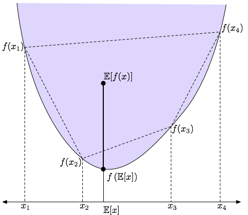
I was quite happy then to have found a graphical “proof” of Jensen’s inequality. By this I mean a proof in the style of the proof of Pythagoras’ theorem that is simply a diagram with the word “Behold!” above it.

Figure 1: Behold! A graphical demonstration of Jensen’s Inequality. The expectations shown are with respect to an arbitrary discrete distribution over the \(x_i\)

Unfortunately, the diagram in Figure 1 is not quite as transparent as the Pythagorean proof so a little discussion is probably required. The diagram shows an instance of Jensen’s inequality for a discrete distribution where the random variable \(x\) takes on one of the \(n\) values \(x_i\) with with probability \(p_i\).

Note that the points \((x_i, f(x_i))\) form the vertices of a polygon which, by the convexity of ƒ, must also be convex and lie within the epigraph of ƒ (the blue shaded area above ƒ). Furthermore, since the \(p_i\) are probabilities they satisfy \(\sum_i p_i = 1\). This means the expected value of the random variable \((x, f(x))\) given by \[ \mathbb{E}[(x, f(x))] = \sum_{i=1}^n p_i \left(x_i, f(x_i)\right) \] is a convex combination and so must also lie within the dashed polygon. In fact, since \(\mathbb{E}[(x, f(x))] = \left(\mathbb{E}[x], \mathbb{E}[f(x)]\right)\) it must lie above \(f\left(\mathbb{E}[x]\right)\) thus giving the result.

Although the diagram in Figure 1 assumes a 1-dimensional space \(X\) the above argument generalises to higher dimensions in an analogous manner. Also, the general result for non-discrete distributions can be gleamed from the provided diagram by a hand-wavy limiting argument. By adding more \(x_i\) to the diagram the dashed polygon the shaded area will approximate the graph of ƒ better. So, by the earlier argument for the discrete case, the expected value of \(x\) will remain within the polygon and thus within the shaded area and thus above ƒ. Since this holds for an arbitrary number of points and nothing weird happens as we take the limit we have the continuous result.

A somewhat surprising fact about Jensen’s inequality is that its converse is also true. By this I mean that if ƒ is a function such that its Jensen gap \(J_f(x)\) is non-negative for all distributions of the random variable \(x\) then ƒ is necessarily convex. The contrapositive of this statement is: ƒ non-convex implies the existence of a random variable \(x\) so that \(J_f(x) < 0\).

Considering Figure 1 again gives some intuition as to why this must be the case. If ƒ was non-convex then its epigraph must, by definition, also be non-convex. This means I could choose some \(x_i\) so that one of the dashed lines lies outside the shaded area. This means I can then choose \(p_i\) so that the mean \(\mathbb{E}[(x, f(x))]\) lies outside the shaded area and thus below the graph of ƒ.

Of course, no self-respecting mathematician would call the above arguments a proof of Jensen’s inequality. There are too many edge cases and subtleties (especially in the continuous case) that I’ve ignored. That said, I believe the statement and thrust of the inequality can be quickly arrived at from the simple diagram above. When using tools like Jensen’s inequality, I find this type of quick insight more valuable than a long, careful technical statement and proof. The latter is valuable to but if I need this level of detail I would look it up rather than try to dredge it up from my sometimes unreliable memory.